Economists prove that the earth is flat

…and in doing so, miss important factors affecting unemployment.

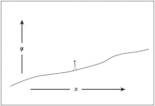
Consider the curve in the diagram below:

Now imagine a man traversing this curve from left to right in small steps of width W. Let us label the exact height (Y) of each foot as YL and YT (L stands for “leading” T stands for “trailing”). The difference in height will clearly depend on the width of the step and the gradient (G) of the slope. This can be expressed as:

 YL = YT + (W x G)

If we now consider smaller and smaller step sizes, in the limit as W approaches zero, YL becomes closer and closer to being equal to YT. If both the gradients and the step sizes are small, a poorly trained mathematician may sloppily pronounce that:

YL = YT        (warning, this equation is wrong)

Hopefully you can see that this statement is wrong, and if taken too seriously could erroneously lead people to believe that “slopes are impossible” and that therefore “the earth is flat”!

So what has this all got to do with economics?

The answer is that many economists have made the same mistake as our proverbial bad mathematician. There is an equation in economics textbooks that states:

aggregate expenditure = aggregate income*

In this case the “leading foot” is aggregate income and the “trailing foot” is aggregate expenditure. This may need some clarification:

The idea that aggregate income equals aggregate expenditure emerges from a simple model of the economy in which all the money that is earned by people is then spent on stuff that was made by people. Or to put it more precisely, the sum total of all the money earned by everyone in the country, per small unit of time (call this unit T), equals the total cost of everything purchased by everyone during that same unit of time. At this point alarm bells should be ringing because you will notice that my explanation of the meaning of the equation involved time, while the equation itself makes no mention of it. Just like the bad mathematician’s equation makes no mention of W. The economists have just said to themselves, “if we make T small enough, we can ignore its effects”. But just like ignoring W, ignoring T, does not allow for any change in the income or expenditure.

So lets see if we can fix this. Looking back at the (correct) equation for the height of the man’s two feet as he traverses x, we should expect the correct form of the expenditure & income equation to have something of the form

aggregate expenditure (at end of interval T) = aggregate income (at start of interval T) + changes in the money supply during T

Anyone that has a clear grasp of our monetary system** will know that loans create money and repayments destroy money. This means that the true state of affairs is as follows:

aggregate expenditure (at end of interval T)  = aggregate income (at start of interval T) + new loans taken out (during past T) – existing loans repaid(during past T)

So what if the original, crude version of the equation is a bit wrong, what problems may this cause?

Answer: you may miss out on the fact that a constantly falling money supply will cause a lack of demand. Aggregate expenditure may be maintained at a level just marginally less than aggregate income for perhaps months or even years.

How does a changing money supply affect the economy?

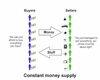
One way you can reasonably model an economy is to imagine that all the buying and selling happens at discreet intervals of duration T, with all the “sellers” of goods doing their selling at one time step and then, being newly armed with money, become buyers at the next step. This is shown in the diagram below for a scenario in which there is a constant money supply. Note the (aggregated) comments made by the parties on each side (click on image for larger version):

Under these circumstances, we can say:

aggregate expenditure (at end of interval T)  = aggregate income (at start of interval T)

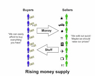
Now consider what will happen in a rising money supply environment in which new money will occasionally be loaned into existence. See the following diagram. Note the comments as well as the additional money shown on the left hand side.

Under these circumstances, we can say:

aggregate expenditure (at end of interval T)  > aggregate income (at start of interval T)

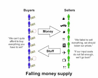
And now by contrast, consider a falling money supply environment in which money will occasionally expire out of existence due to loan repayments. Note the comments as well as the disappearing money shown on the left hand side.

Under these circumstances, we can say:

aggregate expenditure (at end of interval T)  < aggregate income (at start of interval T)

A falling money supply environment is thus likely to be a miserable economic environment with high unemployment. This is why we have all these unconventional money creation schemes (like QE) going on right now. These schemes tend to be described by the media as simply “money printing”, but sadly they are not. Instead they  are all variations of “borrowing money into existence” with a consequence of raising debt levels. So economists and politicians are presenting the public with a false choice between either rising debt or a falling money supply. If economists would consider truly printing money (debt free), then we could have a rising money supply without greater debt.

———————————————
* There are actually alternate versions of this equation which add in factors like investment and foreign trade, but none of these alter the fundamental problem, so I will stick to analysing this most basic version of the equation for the rest of this article. My criticism equally applies to more complex versions of this equation you commonly see in textbooks.
** if you don’t then watch this video.